Juniper Publishers - Novel 3D visualization of Laplace and Fourier transforms
Trends in Technical & Scientific Research

Abstract
This paper will demonstrate how to illustrate poles and zeros of a filter's transfer function as a 3D surface and how this facilitates an understanding of the relationship between the filter's amplitude response and the poles'/zeros' locations in s-space. The transfer function, in Laplace representation, is plotted as a function of the real and imaginary parts of the complex frequency s. This is exemplified for a Chebyshev-II low pass filter.
Keywords: Laplace transform; Poles; zeros; Transfer function; Bode plot; MATLAB; Filter
Abbreviations: PBL: Problem-Based Learning; LTI: Linear Time-Invariant
Introduction
Transforms are probably one of the most versatile engineering tools as they facilitate a visualization of signals in frequency space. The complexity of the subject is widely recognized by students and teachers in engineering disciplines all over the world. It has been suggested that this is due to inconsistencies in the portrayal of transforms in standard textbooks [1]. In order to further the understanding of this abstract subject, different approaches have been suggested. In [2], it was suggested that signals be treated as vectors and transforms should be introduced as a scalar product used to decompose signals in order to disclose signal properties veiled in time space. Other approaches includes PBL (Problem Based Learning) [3] and "conceptual labs” [4,5] and also the use of the proper mathematical tools has been investigated [6].
In this mini review on transforms, a seminal way to graphically visualize poles and zeros that occur in Laplace (and z) transforms as 3D surfaces is suggested. This also facilitates a very elegant means to demonstrate graphically the relationship between the Laplace transform and the Fourier transform.
Discussion
In engineering, Laplace transforms appear for example, as the transfer function in a linear, time-invariant (LTI) system:
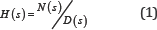
where N(s) and D(s) are polynomials in the complex frequency variable s = s + jw [7]. The roots of the numerator are called zeros and the roots of the denominator are called poles. These are singularities in s-space; at every zero the transfer function has a zero value and at the poles the transfer function has an infinite value. If the polynomial is of order n, there are exactly n poles or zeros, respectively.
Since the frequency variable s is complex, it is a function of both the real part and the imaginary part ω ; H(σ) = H(σ,ω) and |H(σ,w)| is a positive surface in s-space where the poles and zeros will appear as singularities in the surface. For example, let's consider a 3rd order Chebyshev2, low-pass filter with stop band ripple equal to 3 dB:
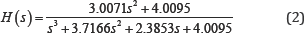
Figure 1 illustrates the Bode diagram of this filter.
The roots of the numerator and denominator are Zeros: 0 ± 1.1547j Poles: -0.1774 ± 1.0776j -3.3619 The poles and zeros are illustrated in a 2D plot in (Figure 2).
This is the traditional way of illustrating poles and zeros. A seminal approach is suggested as follows:
Rewrite the transfer function in (2) as a function of two variables; the real part and the imaginary part;
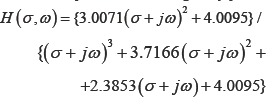
Next, we need to find the absolute value H (σ, w). To this end, an online symbolic computational engine was used [8]. The resulting expression is a square root fraction of polynomials (that is not reproduced here due to limited space). This expression is then used to create a mesh grid in MATLAB which is used to plot a 3D color map of the H(σ, w) function. This is illustrated in (Figure 3) and in (Figure 4) we have zoomed in part of the surface.
First of all we can easily identify the three poles and the two zeros in Figure 3 (compare with Figure 2). Notice what the poles and zeros look like in 3D; poles pull the surface out toward infinity and zeros nail the surface to the “floor”.
The important thing here is to understand how all the graphs in (Figures 1,2 & 3) relate to each other. The relationship between (Figures 2 & 3) should be clear by just comparing the locations of the poles and zeros in the two figures. Relating Figure 1 to the other plots is harder.


The magnitude plot in (Figure 1) represents the filter's amplitude response, i.e. how it responds to harmonics of constant amplitude. In terms of the complex frequency variable s, this corresponds to frequencies with an imaginary part only. The real part of the complex frequency s = σ + jw represents harmonics with exponentially growing/decreasing amplitudes. Hence, the magnitude plot in (Figure 1) corresponds to the cross-section of the 3D surface σ = 0 . Also, in a Bode diagram, only positive frequencies are plotted. So, if we cut the 3D surface in Figure 3 at σ = 0 (= real axis; already done in Figure 3) ω = 0 and at (the imaginary axis), the cross-section edge of the remaining 3D surface is exactly the amplitude response of the filter. In Figure 4 we have plotted the remaining surface and zoomed in on the cross-section edge. Compare the surface edge and the magnitude plot in (Figure 1); they agree exactly.
Conclusion
This work has suggested a seminal way to illustrate poles and zeros of a filter as a 3D plot with the objective of alleviating transform interpretation. From (Figures 3 & 4) the relationship between the pole/zero locations and the filter's amplitude response can be visualized.

It should also be pointed out that since the cross-section edge in Figures 3 & 4 represents σ= 0 , it also represents the magnitude of the Fourier transform, i.e. the Fourier transform of the filter's impulse response; the 3D representation of poles and zeros is also an excellent tool to demonstrate graphically the relationship between the Laplace transform and the Fourier transform.
The same exact technique could be applied to the z-transform with the only difference that the 3D surface should be cut along the unit circle to get the Fourier transform.
To Know More About Trends
in Technical and ScientificResearch Please
click on:
To Know More About Open Access Journals Please click on:


Comments
Post a Comment